Osmosis and Diffusion: Examples, Tonicity, and Practice

Cells and Transport Teaching Resources · High school biology; AP extensions where noted.

Diffusion describes net movement of particles down a concentration gradient due to random molecular motion. Osmosis concerns water movement across a selectively permeable membrane. Osmosis is not the movement of food or wastes into a cell.

Objectives and prerequisites

Students will distinguish diffusion from osmosis, predict initial water movement in a stated situation, and explain dynamic equilibrium. First review solute, solvent, concentration, and selective permeability. Materials: paper and pencil; no lab materials are required for the examples.

Diffusion: separate motion from net movement

Imagine two connected compartments containing a gas at different concentrations. Molecules move in both directions. Initially, more cross from the concentrated side than in the reverse direction, producing net movement down the gradient. At equilibrium the rates balance, but molecular motion continues. Diffusion can occur without a membrane; a membrane adds a permeability constraint.

Osmosis: state the conditions

For a simple classroom prediction, assume equal initial pressure, a membrane permeable to water, and solutes that cannot cross. Water then moves net toward the side with more dissolved nonpenetrating particles. In a fuller explanation, net water movement follows a water-potential difference, and pressure can oppose the solute effect. A cell wall is not the selectively permeable plasma membrane.

Tonicity is a comparison

  • Hypotonic outside solution: lower effective nonpenetrating solute concentration than the cell; net water entry tends to increase cell volume.
  • Hypertonic outside solution: higher effective concentration; water loss tends to reduce cell volume.
  • Isotonic outside solution: no sustained change in cell volume from net water movement under the stated conditions. Water still crosses in both directions.

An animal cell may swell or lyse in a sufficiently hypotonic environment. A plant wall resists expansion, allowing turgor pressure to develop. In a sufficiently hypertonic environment, a plant cell can lose water and its membrane can pull away from the wall: plasmolysis. Equal total solute concentration is not always isotonic when solutes differ in permeability.

Three original practice problems

  1. A cell has 0.15 M nonpenetrating solute; the surrounding solution has 0.30 M. Assume water permeability and equal initial pressure. Predict initial net water movement and classify the surroundings.
  2. A permeable divider separates regions with different oxygen concentrations. What happens to oxygen at equilibrium: do the molecules stop?
  3. Two solutions have equal total solute concentration, but one contains a solute that readily enters the cell. Why might their effects on cell volume differ?

Answer explanations

1: water initially moves net out; the surroundings are hypertonic relative to this cell. 2: molecules continue crossing; opposing rates balance at equilibrium. 3: a penetrating solute can redistribute, changing the effective osmotic difference. Tonicity depends on membrane permeability as well as concentration.

Common misconceptions

Facilitated diffusion is not a backup used only when osmosis stops; different substances can move by different mechanisms simultaneously. Reverse osmosis requires applied pressure and should not be presented as normal spontaneous cellular water movement. Mixing cream into hot coffee also involves bulk fluid motion, so it is not a clean demonstration of diffusion alone.

Teaching note: Have students draw equal arrows in both directions at equilibrium. For AP, ask how increasing pressure on one side changes a water-potential prediction before introducing numerical calculations.

Continue the unit

Sources and further reading

Dihybrid Cross Worksheet: Definition, Examples, Practice & More

Genetics plays a significant role in our understanding of how living organisms come to be as well as bettering our overall knowledge of Biology and cells. Learn more about a dihybrid cross worksheet and the role it plays in genetics. 


Dihybrid Cross Worksheet: Definition, Examples, and Practice


It’s incredible to think that genetics can play a role in how we look, feel, express, and even taste things and it can also play an integral part in what kind of apple grows on a tree, as well as the cells that multiply within us. Genetics is an essential part of understanding all living things and can help us to understand Biology better overall.

Like many aspects of science, genetics is not cut and dry. Often people think they have it all figured out and then become easily confused by another factor. Dihybrid cross is a standard experiment in genetics that students of Biology will study.

We will discuss what it is and help you understand it better, so you can express, explain, and answer any of the questions when your instructor hands you a dihybrid cross worksheet.


What Is A Dihybrid Cross Worksheet?


Dihybrid cross in the “mating experiment between two organisms that are identically hybrid for two characteristics.” What’s a hybrid organism? It’s one that is heterozygous (or monohybrid), which means that it has two different genes (or alleles) at a specific point (this point is often referred to as a locus).

A significant amount of organisms, who can sexually reproduce via the sperm and egg process, have two copies of each gene, which allows them to carry two different alleles. An organism that has parts from two different “true-breeding” lines is often referred to as a hybrid.

While machines or vehicles are not living things, we can easily form a comparison to hybrids; we can also consider this concept when thinking about mixed-breed dogs that have two purebred parents, such as a Puggle or Maltipoo.

The concept and name of the dihybrid cross comes from experimenting with and observing the generations that are produced after two “pure” lines reproduce. A dihybrid cross worksheet allows us to predict how likely an offspring is to inherit a particular single trait.


How to Set Up a Dihybrid Cross Worksheet


A dihybrid cross worksheet will help to predict and determine the genotype of an offspring. It does this by determining all the possible combinations of alleles in the gametes of each of the parents.

As an example, half of the gametes get a dominant S and a dominant Y allele. The other half get a recessive s and a recessive y allele. In this case, both parents are producing 25 percent of each of the following: SY, Sy, sY, and sy.

Since each of the parents, in this case, are producing four different combinations, we must draw a four by four punnett square. We must then list the gametes from one of the parents alone one edge of the punnett square, and the gametes for the other parent along another edge of the punnett square. We will then list in each square, the alleles for the first parent, followed by the addition of the alleles from the second parent. Each combination should contain a dominant-recessive allele. 

The final result will form a diagram of all of the possible combinations of genotypes for the offspring of these two parents.

Try out this method out on a dihybrid cross practice worksheet. 


What is Dominant and Recessive? 


The terms “dominant” and “recessive” refer to the inheritance patterns of certain characteristics. This describes how likely it is for a certain phenotype to be passed on from a parent to their offspring.

Beings that reproduce sexually via the sperm and egg process have two copies of each of their genes. Each of these copies, which are known as alleles, are slightly different and never identical. These differences can affect the rate and variation of proteins that are produced. As proteins affect traits, these differences can affect and produce different phenotypes.

Dominant alleles produce dominant phenotypes and dominant traits in people who have one copy of the allele, which comes from just one parent. In order for a recessive allele to produce a recessive phenotype, the being must have two copies, one from each of the parents. Someone that has a dominant and a recessive allele for a gene will have the dominant phenotype and not the recessive phenotype. This means that they are then considered “carriers” of the recessive allele. This is because the recessive allele is there, however, the recessive phenotype is not.

Dominant and recessive disorders can occur when a person has “broken” genes. This results in a broken code for a protein that doesn’t work properly. Since one regular copy of a gene can mask the effects of a broken gene, many disorders of this type are recessive in their single trait inheritance pattern. However, not all disease alleles are recessive.


Monohybrid Cross Example


A monohybrid cross is defined as a genetic cross mix between individuals who have homozygous genotypes, or genotypes which completely recessive, or completely dominant alleles. This results in opposite phenotypes for a particular genetic characteristic.


Following is an example of a monohybrid cross experiment performed by Gregor Mendel…


Mendel’s Dihybrid Cross Experiment


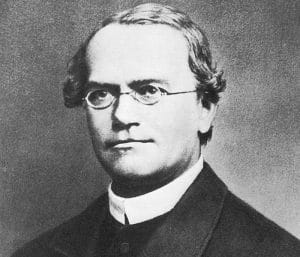
gregor mendel, dihybrid cross worksheet


Gregor Mendel is well known for his work in the field of genetics, and he performed various genetic experiments, including the dihybrid cross, on pea plants in the late 1800s. When he performed dihybrid crosses on plants, he discovered his Law of Independent Assortment.

You might already be familiar with this law of genetics and that it refers to when two or more characteristics are inherited through reproduction, individual hereditary factors independently assort (during gamete or egg production) and give different traits an equal opportunity to occur together.

Even though Mendel was famous for experimenting on pea plants (mostly because the seeds were cheap and readily available), we can consider the dihybrid cross experiment with every living organism from the food we grow to an expanding family.


Let’s observe how Mendel’s Dihybrid Cross experiment looks.


Crossing The P Generation


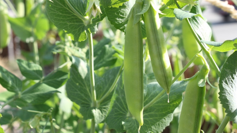
pea plant under sunlight, dihybrid cross worksheet


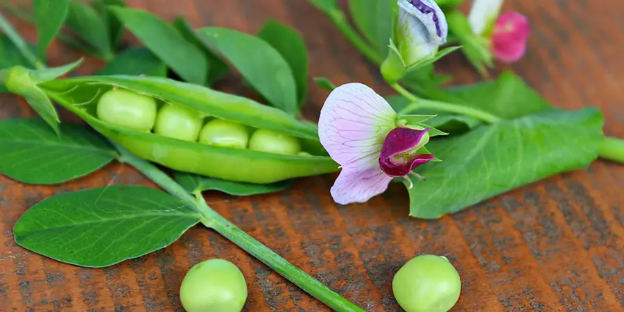
Mendel chose a pea plant that was homozygous and dominant for round (RR) yellow (YY) seeds. He crossed the plant with a pea plant that was homozygous and recessive for wrinkled (rr) green (yy) seeds. Remember, homozygous is a particular gene that has identical alleles.

The notation for crossing the two pea plants is RRYY x rryy. The organisms in this first cross are the parental generation or P generation, which should make sense since they are the “parental” organisms that will be reproducing.

The direct offspring from the P generation (RRYY x rryy cross) is known as the F1 generation. All of the plants from the P generations were heterozygous and had round yellow seeds; the genotype was RrYy.


Crossing The F1 Generation: Dihybrid Cross


The dihybrid cross didn’t occur until Mendel crossed two pea plants from the F1 generation and the notation was RrYy x RrYy. The result of the dihybrid cross gave Mendel the F2 generation and a ratio of 9:3:3:1. Here’s what the ratio means:

  • Nine pea plants with round, yellow seeds
  • Three pea plants with round, green seeds
  • Three pea plants with wrinkled, yellow seeds
  • One pea plant with wrinkled, green seeds

From his findings, Mendel deduced that certain pairs of traits in the P generation sorted independently from one another, from one generation and into the next, and that there is never an equal chance of trait occurrence.


Clarifying The Difference Between A Dihybrid and Monohybrid


Until you get a solid understanding of genetics and cells, dihybrid and monohybrid can be a little confusing, even after we’ve discussed Mendel’s experiment, so let’s clarify the two.

Remember, the dihybrid cross deals with two traits and as the name suggests, the monohybrid centers around a difference in just one trait. The parental organisms are both homozygous for the trait being studied (such as color) but have different alleles for that trait.

One parental organism is homozygous dominant, and the other is homozygous recessive. The F1 generation in a monohybrid is all heterozygous (like the dihybrid cross). F2 generation is typically three-fourths dominant phenotype and one-quarter recessive phenotype.


Applying The Dihybrid Cross Experiment


Mendel’s pea plant dihybrid cross experiment is groundbreaking and helped to form genetics as we know it today, but let’s observe a few other examples…


What Are Some Examples of a Dihybrid Cross Worksheet?


Fruit Flies


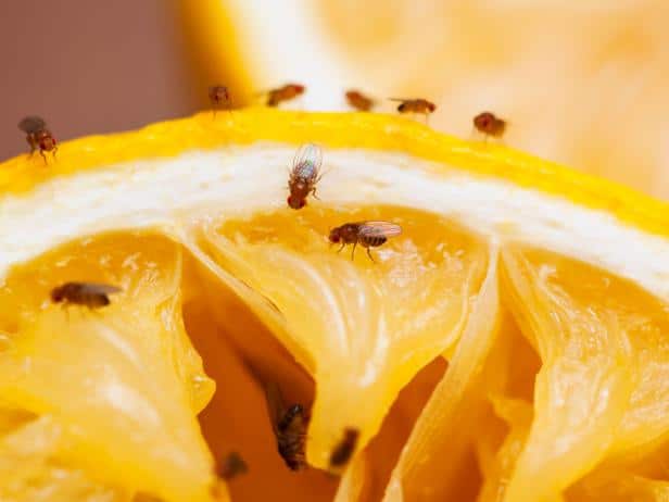
fruit flies, dihybrid cross worksheet


If you were studying fruit flies and wanted to use the dihybrid cross experiment on them, where would you begin? Some may say that you should breed the hybrid flies together while others would recommend counting the number of each type of fruit fly you have.

The first step is to establish the lines of homozygotes. If you want your heterozygotes to breed, you have to ensure that the P generation is “true.”

In order to get a line of homozygotes, you would need to breed the lines repeatedly and select the flies that only show one allele for each characteristic in their offspring. It would be a lengthy process, but that’s the only way a dihybrid cross experiment could be successful.


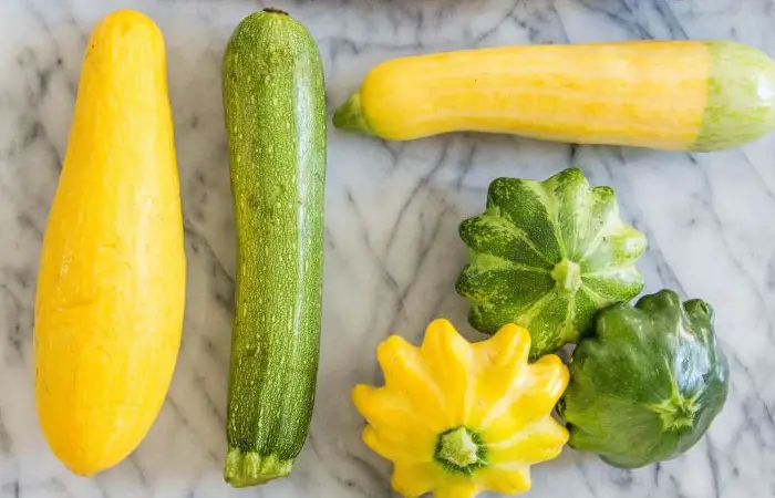
Summer Squash


summer squash, dihybrid cross worksheet


Ready for another example that you might find on a dihybrid cross worksheet? Let’s take a look at this problem.

Find the phenotypic and genotypic ratios for the F1 and F2 generation of summer squash. The summer squash has white fruit color (W), which has dominance over yellow fruit color (w). The disk-shaped fruit (D) has dominance over the sphere-shaped fruit (d).

What results will we have if we cross a squash plant true-breeding for white, disk-shaped fruit with a squash plant true-breeding for yellow, sphere-shaped fruit? Remember, we’re looking for the ratios of F1 and F2 generations.

The P1 geno and phenotypes should be WWDD (white, disk-shaped fruit) x wwdd (yellow, sphere-shaped fruit). To figure out your results, you’ll enter your information into a Punnett Square (you can see how this should look when you click on the genetic cross worksheet that we have listed above).

The results for the F2 generation ratios will form the following:

1:2:2:1:4:2:1:2:1 genotypic ratio (look at the details below)

  • 1/16 will be homozygous dominant for both traits (WWDD)
  • 2/16 will be homozygous dominant for color and heterozygous for shape (WWDd)
  • 2/16 will be heterozygous for color and homozygous dominant for shape (WwDD)
  • 1/16 will be homozygous dominant for color and homozygous recessive for shape (WWdd)
  • 4/16 will be heterozygous for both traits  (WwDd)
  • 2/16 will be heterozygous for color and homozygous recessive gene for shape (Wwdd)
  • 1/16 will be homozygous recessive for color and homozygous dominant for shape (wwDD)
  • 2/16 will be homozygous recessive for color and heterozygous for shape (wwDd)
  • 1/16 will be homozygous recessive for both traits (wwdd)

9:3:3:1 phenotypic ratio (look at the details below)

  • 9/16 will have white, disk-shaped fruit
  • 3/16 will have white, sphere-shaped fruit
  • 3/16 will have yellow, disk-shaped fruit
  • 1/16 will have yellow, sphere-shaped fruit

The Offspring of Made-Up Creatures


Let’s take a look at one more example for variety (and practice).

Imagine a made-up creature that has yellow eyes and green fur. We can assume that both creatures are heterozygous for yellow eyes and green fur, let’s find out the genotype and phenotype of the creature’s offspring; Yellow eyes are E, and green fur is F. The recessive traits are red eyes (ee) and yellow fur (ff). What is the chance that the baby will have red eyes and yellow fur?

First, we need to find the genotype of the parents. Remember that they are heterozygous, which means the genotype is Ee for the eyes and Ff for the fur.

After you form your Punnet Square, you should list every possible combination: E-F, E-f, e-F, e-f. If you’ve filled out your square correctly, there’s a one in 16 chance that the creature’s baby will have red eyes and yellow fur because only one box equals the combination eeff.

As you can see the summer squash problem is a little more complex and time-consuming than Mendel’s pea plant (and the made-up creature is a little bit silly), but with practice and the right information, you can complete any problem on a dihybrid cross worksheet with relative ease and determine the likelihood that certain cells and traits will be produced in an offspring.


Practicing Dihybrid Cross Worksheets


A simple search in Google will bring up many different practice worksheets to help you build upon your skills of creating a dihybrid cross worksheet of your own. Many of these practice worksheets will include a dihybrid cross worksheet answer key so that you can practice yourself and be sure that you are doing them correctly. 

Practicing will ensure that you are ready to answer any questions that your college or university professor may have for you regarding a dihybrid cross worksheet.

Earthworm Dissection: Labeled Anatomy and Lab Guide

Use this earthworm dissection guide to orient a specimen, identify major structures, and explain how its body systems work together. The labeled overview, original specimen images, and observation sequence support a high school biology lab or a diagram-based activity.

Student resources: Earthworm Worksheet and the existing Earthworm Dissection Study Guide (Word). Preview the legacy questions before assigning them; the teaching notes below explain their limits.

Learning goals and materials

  • Distinguish anterior/posterior and dorsal/ventral directions.
  • Trace food from the mouth through the digestive tract to the anus.
  • Use position and connections to identify structures, and separate an observation from an inferred function.

Prerequisites: tissues and organ systems, directional terms, and basic animal classification. Materials: preserved earthworm, dissecting tray, hand lens, blunt probe, forceps, teacher-approved scissors and pins, PPE, and an observation sheet. Use tools appropriate to the specimen and students’ training.

Labeled earthworm anatomy overview

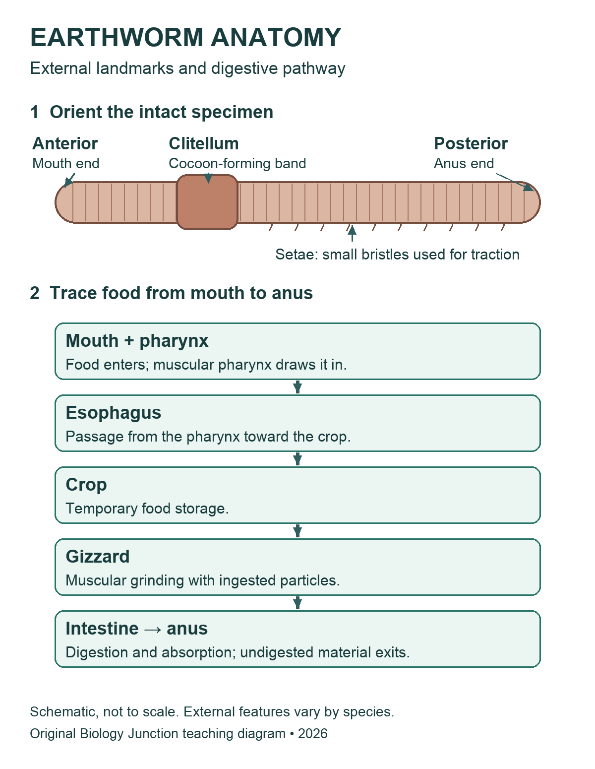
An earthworm is a segmented annelid, not an insect. The mouth is at the anterior end and the anus is at the posterior end. On a mature specimen, the clitellum is closer to the anterior end; confirm orientation using several landmarks.

Earthworm schematic labeling the anterior mouth end, clitellum, posterior anus end and setae, followed by the digestive sequence: mouth and pharynx, esophagus, crop, gizzard, intestine and anus.
Original Biology Junction overview. The body drawing is schematic and does not specify segment counts. Open the image for its full-size version.
Legacy opened-earthworm diagram labeling pharynx, esophagus, crop, gizzard, intestine, dorsal blood vessel and hearts.
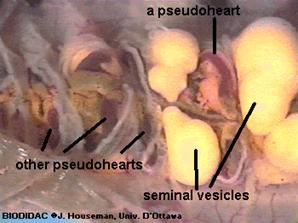
Use this internal view alongside the overview. The legacy label “hearts” refers to aortic arches, not mammalian four-chambered hearts. Open the image for its full-size version.

Existing diagram credit retained: Modern Biology, Holt. Existing photograph credits, including BIODIDAC/J. Houseman, University of Ottawa, remain visible within the original images. The new overview is an original illustration, not a tracing of those figures.

Teacher preparation and safety

Use commercially supplied preserved specimens in a supervised school lab. Before class, review the specimen label, supplier’s safety data sheet (SDS), school risk assessment, ventilation requirements, and storage and disposal procedures. Demonstrate handling and cutting with the actual tools students will use. Require appropriate splash goggles, preservative-compatible gloves, and protective clothing. Keep hands behind the cutting edge and work in a tray. No food or drink.

Rinse or drain a specimen only if the product instructions and school procedure permit it; do not assume preservative belongs in a sink. Report a cut, splash, or spill promptly and follow the lab’s response procedure. Collect tissue, liquids, and sharps as directed, clean the station, and wash hands. A diagram, model, or teacher demonstration can support an alternative activity.

Review the biology lab safety expectations, NSTA’s dissection safety guidance, and the supplier’s specimen FAQs. These general notes do not replace the product-specific procedure.

External anatomy: what to identify first

Lay the intact specimen in the tray. The dorsal surface is usually rounder and darker, and the ventral surface flatter; preservation can alter color. Locate the prostomium, a small lobe over the mouth, then identify segments, the clitellum, and setae. The clitellum is glandular tissue involved in cocoon formation, not an ovary or testis. Tiny reproductive pores may be difficult to see without magnification.

Legacy ventral earthworm drawing showing prostomium, mouth, segments, setae, clitellum and reproductive openings.
Detailed legacy external view. Its segment numbers apply to the illustrated specimen; use a supplier’s species-specific reference rather than treating every label as universal. Open the image for its full-size version.

Many classroom specimens are Lumbricus terrestris, but identify the supplied species from its label rather than appearance alone. Older materials may place earthworms in “Oligochaeta”; current overviews commonly discuss earthworms within Clitellata. Class names and segment landmarks can differ among references.

Teacher-led observation sequence

  1. Orient: sketch the intact specimen and label both ends and dorsal/ventral directions. Record the features used to decide.
  2. Observe externally: use a lens for setae, segments, and clitellum. Do not grade an indistinct pore as though it must be visible.
  3. Open only after demonstration: place the specimen ventral side down. The teacher selects the shallow dorsal opening for the supplied specimen. Lift the body wall away from organs and advance slowly with approved scissors; stop if the tissue layer is unclear.
  4. Expose gently: with guidance, separate only the septa needed to fold back and secure the body wall. Avoid pulling on the digestive tube or dorsal vessel.
  5. Trace before removing: find the pharynx, esophagus, crop, gizzard, and intestine in order. Compare appearance and connections; do not identify an organ by color alone.
  6. Compare systems: locate the dorsal vessel and aortic arches if intact. Examine the ventral nerve cord and nephridia only as directed; moving or removing the gut can damage evidence needed for later observations.
  7. Record uncertainty: label unclear structures “not resolved” and compare with a reference. Finish the class observation sheet, store or dispose as directed, clean the station, and wash hands.

Organs and body systems

Structure What to explain
Crop and gizzard The crop temporarily stores food; the muscular gizzard grinds it with ingested particles. They have different roles.
Intestine Digestion and nutrient absorption occur here. Undigested material leaves through the anus; this is distinct from excretion by nephridia.
Aortic arches and vessels In the familiar Lumbricus lab model, five pairs of aortic arches connect major vessels. The closed circulatory system is distinct from the digestive tube. Use the supplier’s reference for the actual species.
Ventral nerve cord and ganglia A ventral cord connects segmental nervous structures; cerebral ganglia occur near the anterior end. The cord is not a blood vessel.
Nephridia Excretory tubules remove metabolic wastes. They occur in many segments; avoid the absolute claim “two in every segment” for every earthworm.
Reproductive structures Lumbricus has both male and female reproductive organs. Seminal receptacles store sperm received from another worm; the clitellum helps form a cocoon. Not every small structure will be visible in a routine dissection.
Body wall, setae and respiration Circular and longitudinal muscles work with the fluid-supported body; setae provide traction. Gas exchange occurs through the moist body surface, not through lungs.

Teaching notes and original checks

  • Use anatomical landmarks and the supplied species reference before assigning exact segment numbers. The older page’s extra male-pore claim and fixed clitellum range are not suitable universal identification rules.
  • The existing worksheet refers to a dissection ending at segment 32 and to numbered steps from an older procedure. Match those prompts to the procedure actually used; do not assume this revised guide shares the old numbering.
  • Ask students what they could see. A preserved specimen does not demonstrate a heartbeat, feeding, or gas exchange in real time.

Check 1: A student labels the crop “food grinder.” What should change? The gizzard performs muscular grinding; the crop stores food temporarily. Support identification by tracing the connected tract.

Check 2: Is soil passing out of the anus the same process as nephridia removing metabolic wastes? No. Egestion of undigested material and excretion are different processes.

Check 3: Why is an unreadable pore not proof that an organ is absent? Preservation, size, lighting, and the viewing method limit what can be resolved. Record that limitation rather than inventing an observation.

Original specimen and diagram gallery

Compare the existing earthworm photographs and detailed drawings
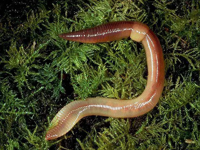
Earthworm on vegetation with clitellum visible.
External specimen photograph. Open the image for its full-size version.
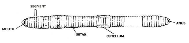
Legacy external earthworm drawing with mouth, segments, setae, clitellum and anus.
External landmarks; proportions and counts are schematic. Open the image for its full-size version.
Legacy close-up of earthworm aortic arches and seminal vesicles.
The photograph uses the older label “pseudohearts.” Open the image for its full-size version.
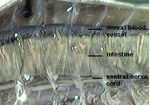
Legacy earthworm photograph labeling dorsal blood vessel, intestine and ventral nerve cord.
Use tissue connections to distinguish the vessel and nerve cord. Open the image for its full-size version.
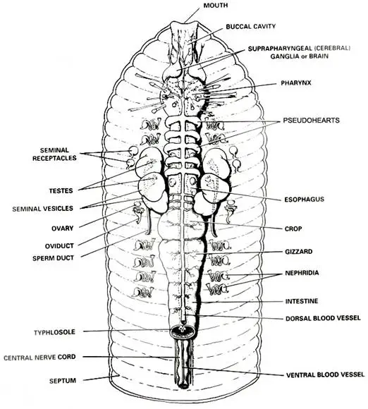
Detailed opened-earthworm drawing with digestive, circulatory, nervous and reproductive structures.
A reference overview; some structures require closer examination than a routine lab permits. Open the image for its full-size version.
Earthworm photograph labeling crop, gizzard, intestine and dorsal blood vessel.
Compare storage and grinding structures. Open the image for its full-size version.
Legacy earthworm diagram showing nephridia, nerve cord, ganglia and digestive organs.
A simplified multi-system view. Open the image for its full-size version.
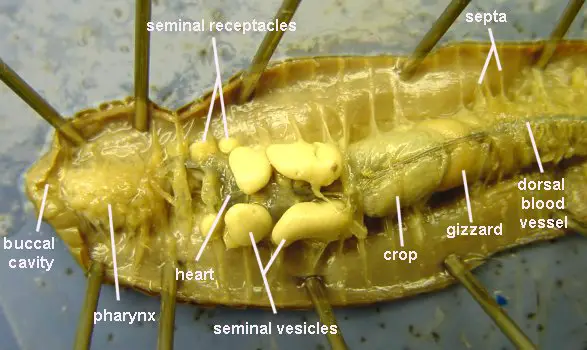
Opened earthworm photograph labeling digestive and reproductive landmarks.
Preview the labels before using this as an observation reference. Open the image for its full-size version.
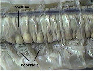
Legacy photograph with intestine and nephridia labeled.
Fine excretory tubules may be difficult to distinguish in a preserved specimen. Open the image for its full-size version.
Legacy earthworm drawing with anterior digestive and reproductive structures and segment numbers.
Numbers belong to this illustration and should be checked against the species supplied. Open the image for its full-size version.
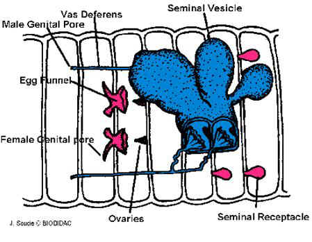
Legacy earthworm reproductive-system diagram.
Compare reproductive structures with the larger digestive landmarks. Open the image for its full-size version.
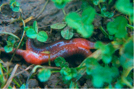
Earthworms together on vegetation.
Existing photograph associated with reproduction; use a reference to interpret the behavior. Open the image for its full-size version.

Related teaching resources and sources

The original checks above are explanations for this guide, not a verified answer key for every legacy worksheet. In the Annelid Review matching section, the esophagus should be described as the passage from the pharynx toward the crop; the supplied “connects the mouth & pharynx” choice needs correction before use. Its class-comparison table also uses historical group names.

Can you do my homework?

Molecular Geometry Chart: Definition, Examples, and Study Guides

How much do you know about molecular geometry definition and the shapes of molecules in chemistry? Join us as we define this subject, go over some examples, and list the different structures you will find in an electron and molecular geometry chart. We have also included some study guides to help you go further.


Molecular Geometry Chart: Definition, Examples, and Study Guides

Molecular geometry is typically taught in college and advanced high school classes. This subject uses geometric models to represent the shape and structure of molecules. It allows scientists to get a precise idea of how the number of atoms and electrons are connected. There are also some rules that help scientists predict which shape a molecule will adopt. There are a huge number of molecules and sequences that can be analyzed. From looking at the number of atoms around a molecule to more difficult structures such as DNA sequence – there are many areas of molecular and electron geometry to explore.


What is a Molecular Geometry Chart?

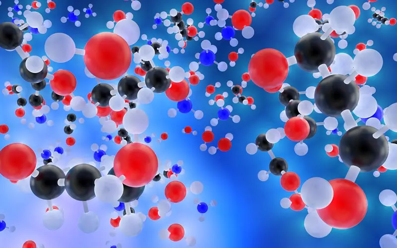
molecular geometry 3d molecules, molecular geometry chart, molecular geometry definition

Molecular geometry is the science of representing molecules in a three-dimensional manner. A molecular geometry chart is a collection of rules on how molecules and electrons will connect and shape a molecule.

Students and scientists can use these charts to create three-dimensional diagrams that represent molecules. These visual representations are interesting because they help students and scientists predict the shape, polarity, and biological activities of a molecule.

These representations can also help with other concepts, such as:

  • Reactivity.
  • Phase of matter.
  • Color.
  • Magnetism.

Molecular geometry can be applied regardless of how complex a molecule is. Students will typically work with simple models at first before learning how to apply these concepts to create detailed models of more complex molecules.


Common Molecular Structures

Molecules obey certain laws when atoms and electrons connect with each other. Molecules will form specific shapes. It is crucial to familiarize yourself with these common shapes so you can determine the correct one.

These are the shapes and structures you will find in a molecular geometry chart:

  • Linear structures.
  • Bent or angular connections.
  • Pyramidal structures.
  • Tetrahedral molecules.

You are probably already familiar with these structures if you have been studying chemistry for a while. Most students have an understanding of these structures thanks to the visual representations of molecules shown in class or textbooks even though they might not know about the rules of molecular geometry.


Polar And Non-Polar Molecules

Certain molecules can be grouped as either polar or non-polar. Other molecules fall between the two.


The geometry of atoms in some molecules is arranged in such a way that one side has a negative charge and the other side has a positive electrical charge. In this case, this type of molecule is called a polar molecule. This means that it has electrical poles. Molecules that aren’t arranged in this way are called non-polar molecules.


Not every molecule that has polar bonds is a polar molecule. For example, carbon dioxide has two polar bonds (C O). However, the molecular geometry of carbon dioxide is linear. This means that the two bonds cancel each other out, resulting in the molecule being non-polar.

Electronegativity

What is electronegativity and why does it vary around a molecular geometry chart? Electronegativity is defined as the measure of the tendency of an atom to attract a bonding pair of electrons.


If two atoms are equally electronegative, then both of those atoms have the same tendency to attract a pair of bonding electrons, and therefore it will be found on average halfway between the two atoms. To get a bond such as this, both atoms would usually be the same atom.


If one of the atoms is slightly more electronegative than the other, this will mean that one of the atoms has a fair share of electron density, and this results in that atom becoming slightly negative. At the same time, the opposing atom will become slightly positive. This is a polar bond.


If one of the atoms is incredibly more electronegative than the other, this will result in the electron pair being dragged right over to that electronegative atom. This means that the other atom loses all control of its electron, and the electronegative atom has complete control over both electrons. This results in ions being formed and is called an ionic bond.


Lewis Theory And Valence-Shell Electron-Pair Repulsion Theory

You can’t gain a thorough understanding of molecular geometry without studying the Lewis theory and the Valence-shell electron-pair repulsion theory.

The Lewis theory is about how valence shell electrons bond with an atom. This approach represents atoms and electrons in a two-dimensional manner. You will often start with this simple visual representation called a Lewis structure to determine the correct three-dimensional structure for a molecule.

You can create a Lewis structure electron dot diagram by simply writing the symbol for the atom you want to represent. You would then add dots to represent the valence shell electrons connected to the atom.

A valence electron is an electron located in the outer shell of the atom. It is common to omit the electrons that aren’t connected to the outer shells of an atom since they won’t form bonds with other elements and would only make Lewis structure diagrams more complicated. If a shell is closed, the electrons that can be found in this shell won’t be shown on a Lewis electron dot diagram.

In a Lewis structure, you can place the dots on any side of the symbol. However, you can’t have more than two dots per side.

The Valence shell electron-pair repulsion theory states that electrons will naturally repel each other. This applies regardless of the type of pairs they form.

Electrons can form bonded pairs, lone pairs, double bonds, triple bonds, or exist as single unpaired electrons. They will position themselves around an atom so that there is as much space as possible between them. In molecular geometry, each pair or single unpaired electron counts as an electron group.

This natural behavior reduces repulsion between electrons and maximizes the space available to attract other elements the electrons can bond with.

The Valence-shell electron-pair repulsion theory is important vital in the context of molecular geometry because it will help you figure out the angle of the different bonds that exist around an atom. You can use this theory to deduce the structure of a molecule.


Molecular Geometry Structures And Atom Groups

You can determine the structure and shape of a molecule once you know about the atoms that make up this molecule, how many electrons are connected to these atoms, and which type of bond these electrons form.

These are the different structures molecules can adopt:

  • If you have an atom with two electron groups, the molecule will adopt take a linear structure.
  • If you have three electron groups, you will have a trigonal-planar structure.
  • The molecule will adopt a bent structure if there are three groups of electrons with a lone pair.
  • If there are four groups of electrons, the molecule will have a tetrahedral shape.
  • A molecule with four groups of electrons and a lone pair of electrons will take the shape of a trigonal pyramid.
  • If you have four groups of electrons and two lone pairs, the molecule will have a bent structure.
  • A molecule with five electron groups will adopt a trigonal-bipyramidal structure.
  • If there are five electron groups and a lone pair of electrons, the molecule will have a seesaw structure.
  • A molecule with five electron groups and two lone pairs, the molecule will be T-shape shaped.
  • If there are five electron groups and three lone pairs, you will have a linear structure.
  • A molecule with six electron groups will have an octahedral shape.
  • A molecule with six electron groups and a lone pair will be shaped like a square pyramid.
  • If you have six electron groups and two lone pairs, the molecule will adopt a square planar structure.

These thirteen different scenarios cover all the different structures you will encounter in molecular geometry. You don’t need to learn them by heart since you can easily deduct the structure that makes the most sense by applying the Valence-shell electron-pair repulsion theory.


Molecules With More Than One Atom
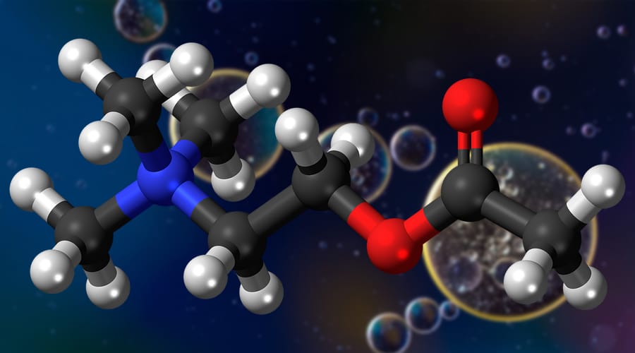
blue and red molecules, molecular geometry chart, molecular geometry definition

The molecular geometry chart still applies if you have a molecule with more than one atom. The structure will be more complex and will probably combine different geometric shapes.

If you have a complex molecule, break it down into smaller section and look at each atom individually. Determine how the electrons will connect to this atom in function of the type of bond they form and of the number of electron groups.

You can use molecular geometry rules to determine the shape and structure of each atom and its electrons. You can then apply the Valence-shell electron-pair repulsion theory to determine how these different small structures will connect to each other to form a more complex molecule.


Ions

An ion is defined as a molecule or atom which has acquired an electrical charge due to gaining or losing electrons. Polyatomic ion charges are ones which are composed of two or more atoms. When a polyatomic ion is involved in a chemical reaction, the oxidation number of it plays a significant role. This is a number which is either negative, positive, or zero. This oxidation number is an indication of the number of electrons in which an ion can share, lose, or gain when chemically reacting which an atom, compound, molecule, or with another ion. The oxidation number of a polyatomic ion is worked out at the sum of the oxidation numbers that belong to its constituent atoms. This is equal to the positive charge, negative charge or neutral charge that exists on the ion.


Diatomic Molecules

A diatomic molecule consists of two atoms. The majority of diatomic molecules are ones of the same element, however, a few combine different elements. Most diatomic molecules are gases at room temperature.


Octahedral Molecular Geometry

Octahedral molecular geometry refers to the shape of the compounds that have six atoms or ligands symmetrically arranged around a central atom. This defines the vertices of an octahedral shape. The octahedron is platonic solid, even though octahedral molecules tend to have a central atom and no bonds. The term “octahedral” is a loosely used term amongst scientists, as it focuses purely on the geometry of bonds to the central atom, rather than looking at the differences in the ligands.


Bond Angles And Three-Dimensional Geometry

Students often make the mistake of thinking in two dimensions when determining bond angles. Electrons will position themselves to be as far away from each other as possible, but keep in mind that they will do this on a three-dimensional plane. A molecular geometry chart with bond angles will help to clarify these structures.

Working with three-dimensional models is a great way to get used to thinking about geometry in a three-dimensional plane. There are also apps and software you can use to create virtual models and get used to these concepts.

What is the Difference Between Electron-Pair Geometry and Molecular Structure?

Electron Geometry

Electron geometry is the term used for the geometry of the electron pair located on the central atom. This applies whether they are bonding electrons or non-bonding electrons. The definitions of an electron pair is electrons that are in pairs or multiple bonds, lone pairs and sometimes even just one single electron that is unpaired. Electrons are always in constant motion and it can be difficult to determine the path that they are going to take. With this in mind, the arrangement of electrons within a molecule is defined by electron density distribution.


An Example of Electron Geometry

We will use CH4 as an example.


The central atom in this example is C, plus there are also four valence shell electrons. The hydrogen atoms give four electrons, so that means that there are a total of eight electrons around C. In this example, the single number of bonds are four, and the number of lone pairs here is zero. So with this in mind, we can determine here that the electron geometry of CH4 is tetrahedral.


Molecular Geometry

Molecular geometry is the term used when determining the shape of a molecule. This refers to the three-dimensional structure or arrangement of the atoms within a molecule. There is usually a central atom which is surrounded by electrons. When we understand the molecular geometry of a compound, this makes it much easier to determine the magnetism, phase of matter, polarity, color, and reactivity of that compound. The geometry of molecules is often described using bond lengths, bond angles, and torsional angles. With smaller molecules, simply the molecular formula, along with a table of angles and standard bond lengths may be all that is needed to determine the geometry of that particular molecule. It is predicted by looking at only the electron pairs, which is what makes molecular geometry different from electron geometry.


An Example of Molecular Geometry

We will use H2O as an example.

H2O is a common polar molecule. The central atom in this case is the oxygen atom which has six valence electrons. Hydrogen, in this case, gives a total of two electrons, which makes the total overall amount of electrons eight. In this example, there are two lone electron pairs, and four electron groups, as well as two single bond pairs. Therefore, the molecular geometry in this example is bent.


Why Do Most Atoms Form Chemical Bonds?


Most elements contain atoms that form chemical bonds. This is because those atoms become more stable when they are bonded together. Neighbouring atoms are attracted to each other by electrical forces which make them stick together. Atoms that are strongly attractive rarely spend much time on their own – other atoms will usually bond to them quite quickly. The arrangement of electrons around a central atom is what determines the strength in which it seeks out other atoms to bond with.  


Chemical Bonds

A chemical bond is formed by the joining of two or more atoms. A stable compound occurs when the total energy of the combined atoms has lower energy than if the atoms were separate. The combined state of these atoms implies there is an attractive force between these atoms – a chemical bond. There are two extreme cases of chemical bonds. These are covalent formula bonds and ionic formula bonds.


Covalent Bonding

A covalent formula bond is one which involves sharing of valence electrons by two atoms. These types of covalent bonding can create stable molecules, as long as they share electrons in a way that creates noble gas electron configuration for each atom.


Ionic Bonds

During chemical bonds, atoms can either share or transfer their valence electrons. In some extreme cases, one or more atoms may lose electrons and then other atoms gain them which produces noble gas electron configuration. The bond in this case is called an ionic bond.


What Is The Difference Between Atomic Orbitals And Molecular Orbitals?


The orbital is a region in which the probability of finding an electron is relatively higher than usual. Atoms have a nucleus and within this nucleus they have their own electrons rotating around. When orbitals are overlapped to create molecules via bonding, these types of orbitals are named molecular orbitals. Molecular orbital theory and valence bond theory both explain the properties of molecular and atomic orbitals. Orbitals can hold two electrons within them maximum. The main difference between molecular orbital calculation and atomic orbital calculation is that electrons within a molecular orbital are influenced by two or more nuclei. This depends on the number of atoms in the molecule. Atomic orbitals are different as they are only influenced by one positive nucleus.


Organic Chemistry


Organic chemistry refers to the study of the composition, structure, properties, preparation, and reactions of compounds which contain carbon. This includes compounds that are not only hydrocarbons, but also compounds which contains a number of other elements such as hydrogen, oxygen, halogens, nitrogen, phosphorus, sulfur, and silicon. This type of chemistry used to only refer to compounds that were produced by living beings. However, it has now been broadened to focus on other substances such as plastics. There is a huge range of organic compounds and these include things such as food, explosives, paints, cosmetics, and pharmaceuticals. Organic chemistry is the best way of creating new compounds. Scientists will develop new and better ways of synthesizing existing compounds with organic chemistry.


Study Guides

There are several study guides on molecular geometry chart information which you can use to go further and practice molecular geometry. This subject gets easier once you start applying it and become familiar with all the different structures molecules can adopt.

You should start by modeling simple molecules or look at three-dimensional models of different molecules to identify their shape and ask yourself what kind of atom groups and bond types caused the molecule to adopt this structure.

Here are a few study guides to help you go further:

  • This study guide from NYU covers the basics and includes some helpful diagrams of the most common shapes you encounter. We like that the angles are indicated for each diagram.
  • This study guide from Angelo University goes over the Lewis structures, the types of bonds you will encounter, and talks about exceptions and resonance structures. There are plenty of examples, and this material will help you explore additional concepts.
  • This molecular geometry guide from Oklahoma State University sums up all the different structures with a detailed table. This is a great resource if you need help with understanding how angles are determined.
  • This comprehensive guide explores the Lewis dot structures and shows you how to place the dots around the atom symbols.
  • You can test your molecular geometry knowledge with these flashcards and quiz questions.

Interactive 3D Tool

The University of Colorado has an online interactive tool that lets you create 3D models of different molecules. You can select different types of electron groups and see how they will connect to an atom.

This tool will show you the angle of the bonds and show models for different molecules if you don’t want to create one from scratch.

This visual tool would be very useful in a classroom when teaching molecular geometry chart information, but you can use it to try and recreate the thirteen different structures that exist in molecular geometry or to try recreating different specific molecules.

Molecular geometry is a fascinating subject. Studying molecular geometry can seem complex at first, but things become easier once you become familiar with the different structures that exist and understand which factors will influence how a molecule is shaped. Make good use of the study guides listed above, and take the time to play with the interactive 3D tool to try different things.

 

Everything You Need to Know About the Calvin Cycle

The Calvin Cycle occurs during photosynthesis and consists of light independent redox reactions that convert carbon dioxide into glucose. This conversion happens in the chloroplast, or more specifically the stroma of the chloroplast. The chloroplast region is an area between the thylakoid membrane and the inner membrane of the organelle which is typically located in the leaves of plants.

This cycle used to create carbon sugars, mostly, was discovered by Melvin Calvin, Andrew Benson, and James Bassham in 1950 at the University of California. The used radioactive material to trace the pathways carbon atoms took during the carbon fixation step in plant life.

You’ve probably heard the Calvin Cycle called a few other names including the CBB Cycle, C3 Cycle, and dark reactions to name a few.

This process of carbon fixing by plants is essential to all life on the planet. Most new organic growth stems from plants converting carbon to sugars either directly or indirectly. Other plants, or animals, can use these sugars to forms more complex sugars and amino acids when they consume them. It all stems from little plants working day and night to capture light and water.

A Technical Take on the Calvin Cycle

The Calvin Cycle

The Calvin Cycle occurs during photosynthesis and is repeated until it forms a glucose molecule. Photosynthesis goes through two stages to create food and building materials for plants to grow. During the first stage, chemical reactions from light produce ATP and NADPH. The second stage is when the Calvin Cycle takes place. In this stage, carbon dioxide and water get converted to organic materials like glucose. These reactions are called dark reactions which confuses people, but they do not take place at night.

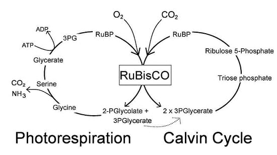
The short explanation of the Calvin Cycle is that it begins with carbon fixation. Carbon dioxide molecules are plucked out of the air to produce glyceraldehyde 3-phosphate. RuBisCO, an enzyme found abundantly around the planet, brings on the carboxylation of a 5-carbon compound and provides a 6-carbon compound that halves itself form two 3-phosphoglycerate. The enzyme phosphoglycerate kinase uses the phosphorylation to create biphosphoglycerate.

Next, the enzyme glyceraldehyde 3-phosphate dehydrogenase uses the reduction of biphosphoglycerate by NADPH. This is called the reduction reactions. Eventually, when the cycle ends, the reactions and reductions produce one glyceraldehyde 3-phosphate molecule per every three carbon dioxide molecules.

That’s a lot of massive words. What that means is the plant uses light and water to convert carbon dioxide into nutrients and oxygen. It takes six turns on the Calvin Cycle for the plant to produce a single glucose molecule. Now that we simplified the process, let’s look at the chemical equation for the Calvin Cycle:

3 CO2 + 6 NADPH + 5 H2O + 9 ATP → glyceraldehyde-3-phosphate (G3P) + 2 H+ + 6 NADP+ + 9 ADP + 8 Pi (Pi = inorganic phosphate)

The Simplified Function of the Calvin Cycle

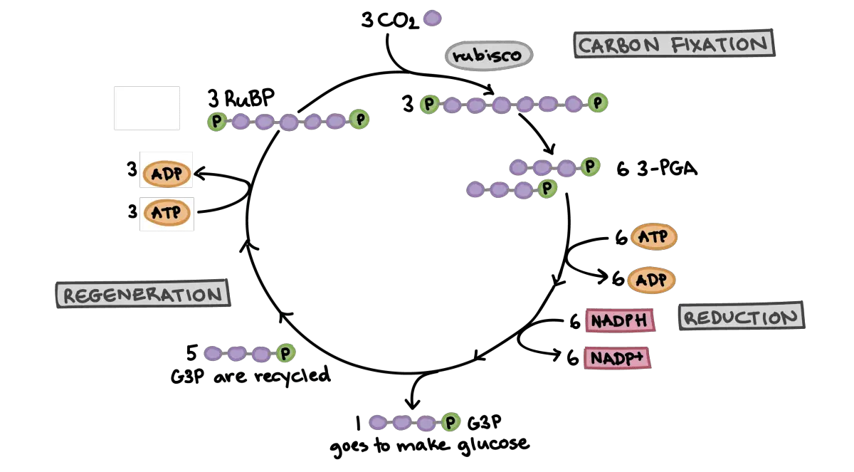
Simplified-Calvin-Cycle-diagram

How plants create sugar from sunlight, water, and carbon dioxide is complicated as you probably noted from the previous section. However, plants toil away day and night creating glucose, starch, and cellulose so they can grow. The Calvin Cycle plucks carbon molecules right out of the air and creates new plant growth.

The Calvin Cycle is vital to every ecosystem, and it reaches far beyond the plants using it. Plants are the building blocks of all the food in any ecosystem. Herbivores eat plants for energy and growth while carnivores eat herbivores for the same reasons. In the end, everything goes back into the ground and plants start the process all over again.

If plants stopped all their hard work tomorrow, it would only take a few days for animals to start feeling the effects and starving. Herbivores lose their food right away. Carnivores would follow behind the herbivores. Plants make most of the basic building blocks we all need to continue life as we know it. Without their hard work, we’d all be doomed.

While plants are supplying us with the building blocks, we need to continue living, and they help out the environment in other ways. Because the Calvin Cycle depends on carbon dioxide, plants indirectly play a role in regulating carbon dioxide and other gases proven to be harmful to the atmosphere. Plants perform an essential role in helping us clean the air we breathe.

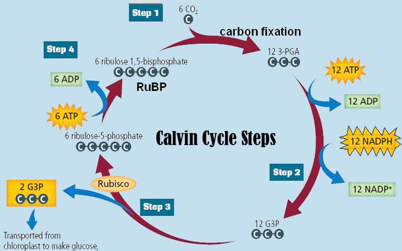
The Calvin Cycle Step by Step

Calvin Cycle step by step

Carbon fixation is the first step. We explained it in brutal technical detail above, but let’s look at it in simpler terms in this section. A carbon dioxide molecule is plucked from the air and combined with a five-carbon acceptor molecule called ribulose-1,5-bisphosphate, or RuBP for short. The result is a six-carbon molecule.

The six-carbon molecule is split in half to form a set of new carbon molecules called 3-phosphoglyceric acid, or 3-PGA for short. The new three-carbon molecules are catalyzed by an enzyme called RuBisCo. This creates the simple sugar molecules the Calvin Cycle needs for stage two. On a side note, because it is used by every plant during photosynthesis, the RuBisCo enzyme if the most common catalyst on Earth. The result of this step is passed on to the next phase.

Step two of the Calvin Cycle is called the reduction step. The 3-PGA molecules created in the carbon fixation step are used in phase two to develop glyceraldehyde-3 phosphate or G3P for short. G3P is a simple sugar. This process uses energy and reactions captured during light-dependent stages of photosynthesis.

This step is called the reduction step because electrons are stolen from molecules created during photosynthesis and given to our new sugars. In chemistry, when you take electrons from a molecule, it’s called a reduction hence the name of this stage. Technically, the electrons are donated and not taken. Taking electrons by force is called oxidation, and that’s not what happens in this stage.

At this point, our plant has created sugar it can store for a long time and use for energy. Anything that eats this plant gets to take advantage of these sugars as well including humans. The plant may choose to use these stored molecules to form new plant materials or repair itself, but that’s not part of the Calvin Cycle so we won’t get into it. This is the end of the sugar-producing phase of the Calvin Cycle.

The final stage of the Calvin Cycle is called the regeneration step. Some of the G3P are held back and not used to make sugars. Instead, they are used to revitalize the five – carbon compound the Calvin Cycle needs to start the process over again. It takes six carbon molecules to make glucose, so plants have to go through the Calvin Cycle six times to make one glucose molecule.

Once the plant has completed this cycle six times, the Calvin Cycle ends and begins again. So, technically, the Calvin Cycle is all three steps done six times each. Plants repeat this process over and over during daylight hours. At night they continue to work making various compounds that don’t require light. This makes plants the most efficient lifeforms on the planet.

Bonus Information About Plants and Their Internal Food Factories

plants

We usually consider waste products bad or at least not edible. However, we need the waste materials plants to produce to survive. An essential waste, or by-product, plants produce is oxygen. While plants are using water and carbon dioxide to make sugars, they release oxygen into the air around them as a waste product.

The delicious fruits and vegetables we all enjoy get most of their flavor from the carbon sugars plants store for energy. From the crunchy stalk of the celery plant to the succulent meat of the peach, plants developed all using just carbon dioxide, water, sunlight, and a few minerals leeched from the soil. I think we can assume these tasty treats are little gifts from the plant kingdom.

The tiny organelles called chloroplasts on the surface of a plant’s leaves can move. Ok, they can’t move individually, but in many plants, they can turn the leaf, so it gets better exposure to sunlight. These plant-based solar cells help capture sunlight so being able to point yourself in the sun makes sense. Some plants take it to another level and bend their stalk or branches to help reach the sunlight.

Some Final Notes

photosynthesis diagram

The fantastic plants we ignore all around us are vital to our survival. They use energy from the Sun in little energy reactors called chloroplasts to do all sorts of cool things. If you glance at the bigger picture and oversimplify it, plants take light from the Sun and turn it into carbon sugars they can store for long periods of time. We could call them solar powered batteries if we want to be humorous about the process.

Plants pitch in and help everywhere they can from cleaning the air to enriching the soil they grow in for the next plants. Plants give us so many things from apples to steak. Without plants toiling away at the bottom of the food chain, nothing in the top of the food chain could survive. Every food we consume comes from plants either directly or indirectly.